
I’ve been reading papers about deep learning for several years now, but until recently hadn’t dug in and implemented any models using deep learning techniques for myself. To remedy this, I started experimenting with Deeplearning4J a few weeks ago, but with limited success. I read more books, primers and tutorials, especially the amazing series of blog posts by Chris Olah and Denny Britz. Then, with incredible timing for me, Google released TensorFlow to much general excitement. So, I figured I’d give it a go, especially given Delip Rao’s enthusiasm for it—he even compared the move from Theano to TensorFlow feeling like changing from “a Honda Civic to a Ferrari.”
Here’s a quick prelude before getting to my initial simple explorations with TensorFlow. As most people (hopefully) know, deep learning encompasses ideas going back many decades (done under the names of connectionism and neural networks) that only became viable at scale in the past decade with the advent of faster machines and some algorithmic innovations. I was first introduced to them in a class taught by my PhD advisor, Mark Steedman, at the University of Pennsylvania in 1997. He was especially interested in how they could be applied to language understanding, which he wrote about in his 1999 paper “Connectionist Sentence Processing in Perspective.” I wish I understood more about that topic (and many others) back then, but then again that’s the nature of being a young grad student. Anyway, Mark’s interest in connectionist language processing arose in part from being on the dissertation committee of James Henderson, who completed his thesis “Description Based Parsing in a Connectionist Network” in 1994. James was a post-doc in the Institute for Research in Cognitive Science at Penn when I arrived in 1996. As a young grad student, I had little idea of what connectionist parsing entailed, and my understanding from more senior (and far more knowledgeable) students was that James’ parsers were really interesting but that he had trouble getting the models to scale to larger data sets—at least compared to the data-driven parsers that others like Mike Collins and Adwait Ratnarparkhi were building at Penn in the mid-1990s. (Side note: for all the kids using logistic regression for NLP out there, you probably don’t know that Adwait was the one who first applied LR/MaxEnt to several NLP problems in his 1998 dissertation “Maximum Entropy Models for Natural Language Ambiguity Resolution“, in which he demonstrated how amazingly effective it was for everything from classification to part-of-speech tagging to parsing.)
Back to TensorFlow and the present day. I flew from Austin to Washington DC last week, and the morning before my flight I downloaded TensorFlow, made sure everything compiled, downloaded the necessary datasets, and opened up a bunch of tabs with TensorFlow tutorials. My goal was, while on the airplane, to run the tutorials, get a feel for the flow of TensorFlow, and then implement my own networks for doing some made-up classification problems. I came away from the exercise extremely pleased. This post explains what I did and gives pointers to the code to make it happen. My goal is to help out people who could use a bit more explicit instruction and guidance using a complete end-to-end example with easy to understand data. I won’t give lots of code examples in this post as there are several tutorials that already do that quite well—the value here is in the simple end-to-end implementations, the data to go with them, and a bit of explanation along the way.
As a preliminary, I recommend going to the excellent TensorFlow documentation, downloading it, and running the first example. If you can do that, you should be able to run the code I’ve provided to go along with this post in my try-tf repository on Github.
Simulated data
As a researcher who works primarily on empirical methods in natural language processing, my usual tendency is to try new software and ideas out on language data sets, e.g. text classification problems and the like. However, after hanging out with a statistician like James Scott for many years, I’ve come to appreciate the value of using simulated datasets early on to reduce the number of unknowns while getting the basics right. So, when sitting down with TensorFlow, I wanted to try three simulated data sets: linearly separable data, moon data and saturn data. The first is data that linear classifiers can handle easily, while the latter two require the introduction of non-linearities enabled by models like multi-layer neural networks. Here’s what they look like, with brief descriptions.
The linear data has two clusters that can be separated by a diagonal line from top left to bottom right:
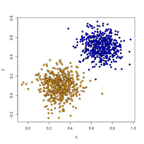
Linear classifiers like perceptrons, logistic regression, linear discriminant analysis, support vector machines and others do well with this kind of data because learning these lines (hyperplanes) is exactly what they do.
The moon data has two clusters in crescent shapes that are tangled up such that no line can keep all the orange dots on one side without also including blue dots.
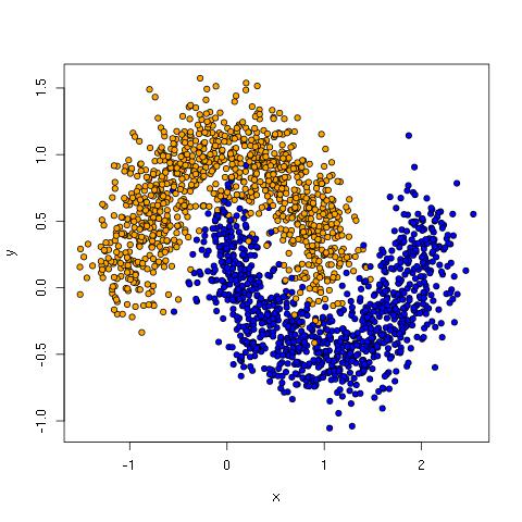
Note: see Implementing a Neural Network from Scratch in Python for a discussion working with the moon data using Theano.
The saturn data has a core cluster representing one class and a ring cluster representing the other.
With the saturn data, a line is catastrophically bad. Perhaps the best one can do is draw a line that has all the orange points to one side. This ensures a small, entirely blue side, but it leaves the majority of blue dots in orange terroritory.
Example data has been generated in try-tf/simdata for each of these datasets, including a training set and test set for each. These are for the two dimensional cases visualized above, but you can use the scripts in that directory to generate data with other parameters, including more dimensions, greater variances, etc. See the commented out code for help to visualize the outputs, or adapt plot_data.R, which visualizes 2-d data in CSV format. See the README for instructions.
Related: check out Delip Rao’s post on learning arbitrary lambda expressions.
Softmax regression
Let’s start with a network that can handle the linear data, which I’ve written in softmax.py. The TensorFlow page has pretty good instructions for how to define a single layer network for MNIST, but no end-to-end code that defines the network, reads in data (consisting of label plus features), trains and evaluates the model. I found writing this to be a good way to familiarize myself with the TensorFlow Python API, so I recommend trying it yourself before looking at my code and then referring to it if you get stuck.
Let’s run it and see what we get.
$ python softmax.py --train simdata/linear_data_train.csv --test simdata/linear_data_eval.csv
Accuracy: 0.99
This performs one pass (epoch) over the training data, so parameters were only updated once per example. 99% is good held-out accuracy, but allowing two training epochs gets us to 100%.
$ python softmax.py --train simdata/linear_data_train.csv --test simdata/linear_data_eval.csv --num_epochs 2
Accuracy: 1.0
There’s a bit of code in softmax.py to handle options and read in data. The most important lines are the ones that define the input data, the model, and the training step. I simply adapted these from the MNIST beginners tutorial, but softmax.py puts it all together and provides a basis for transitioning to the network with a hidden layer discussed later in this post.
To see a little more, let’s turn on the verbose flag and run for 5 epochs.
$ python softmax.py --train simdata/linear_data_train.csv --test simdata/linear_data_eval.csv --num_epochs 5 --verbose True
Initialized!

Training.
0 1 2 3 4 5 6 7 8 9
10 11 12 13 14 15 16 17 18 19
20 21 22 23 24 25 26 27 28 29
30 31 32 33 34 35 36 37 38 39
40 41 42 43 44 45 46 47 48 49

Weight matrix.
[[-1.87038445 1.87038457]
[-2.23716712 2.23716712]]

Bias vector.
[ 1.57296884 -1.57296848]

Applying model to first test instance.
Point = [[ 0.14756215 0.24351828]]
Wx+b = [[ 0.7521798 -0.75217938]]
softmax(Wx+b) = [[ 0.81822371 0.18177626]]

Accuracy: 1.0
Consider first the weights and bias. Intuitively, the classifier should find a separating hyperplane between the two classes, and it probably isn’t immediately obvious how W and b define that. For now, consider only the first column with w1=-1.87038457, w2=-2.23716712 and b=1.57296848. Recall that w1 is the parameter for the `x` dimension and w2 is for the `y` dimension. The separating hyperplane satisfies Wx+b=0; from which we get the standard y=mx+b form.
Wx + b = 0
w1*x + w2*y + b = 0
w2*y = -w1*x – b
y = (-w1/w2)*x – b/w2
For the parameters learned above, we have the line:
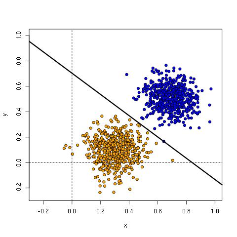
y = -0.8360504*x + 0.7031074
Here’s the plot with the line, showing it is an excellent fit for the training data.
.
The second column of weights and bias separate the data points at the same place as the first, but mirrored 180 degrees from the first column. Strictly speaking, it is redundant to have two output nodes since a multinomial distribution with n outputs can be represented with n-1 parameters (see section 9.3 of Andrew Ng’s notes on supervised learning for details). Nonetheless, it’s convenient to define the network this way.
Finally, let’s try the softmax network on the moon and saturn data.
python softmax.py --train simdata/moon_data_train.csv --test simdata/moon_data_eval.csv --num_epochs 2
Accuracy: 0.856

$ python softmax.py --train simdata/saturn_data_train.csv --test simdata/saturn_data_eval.csv --num_epochs 2
Accuracy: 0.45
As expected, it doesn’t work very well!
Network with a hidden layer
The program hidden.py implements a network with a single hidden layer, and you can set the size of the hidden layer from the command line. Let’s try first with a two-node hidden layer on the moon data.
$ python hidden.py --train simdata/moon_data_train.csv --test simdata/moon_data_eval.csv --num_epochs 100 --num_hidden 2
Accuracy: 0.88
So,that was an improvement over the softmax network. Let’s run it again, exactly the same way.
$ python hidden.py --train simdata/moon_data_train.csv --test simdata/moon_data_eval.csv --num_epochs 100 --num_hidden 2
Accuracy: 0.967
Very different! What we are seeing is the effect of random initialization, which has a large effect on the learned parameters given the small, low-dimensional data we are dealing with here. (The network uses Xavier initialization for the weights.) Let’s try again but using three nodes.
$ python hidden.py --train simdata/moon_data_train.csv --test simdata/moon_data_eval.csv --num_epochs 100 --num_hidden 3
Accuracy: 0.969
If you run this several times, the results don’t vary much and hover around 97%. The additional node increases the representational capacity and makes the network less sensitive to initial weight settings.
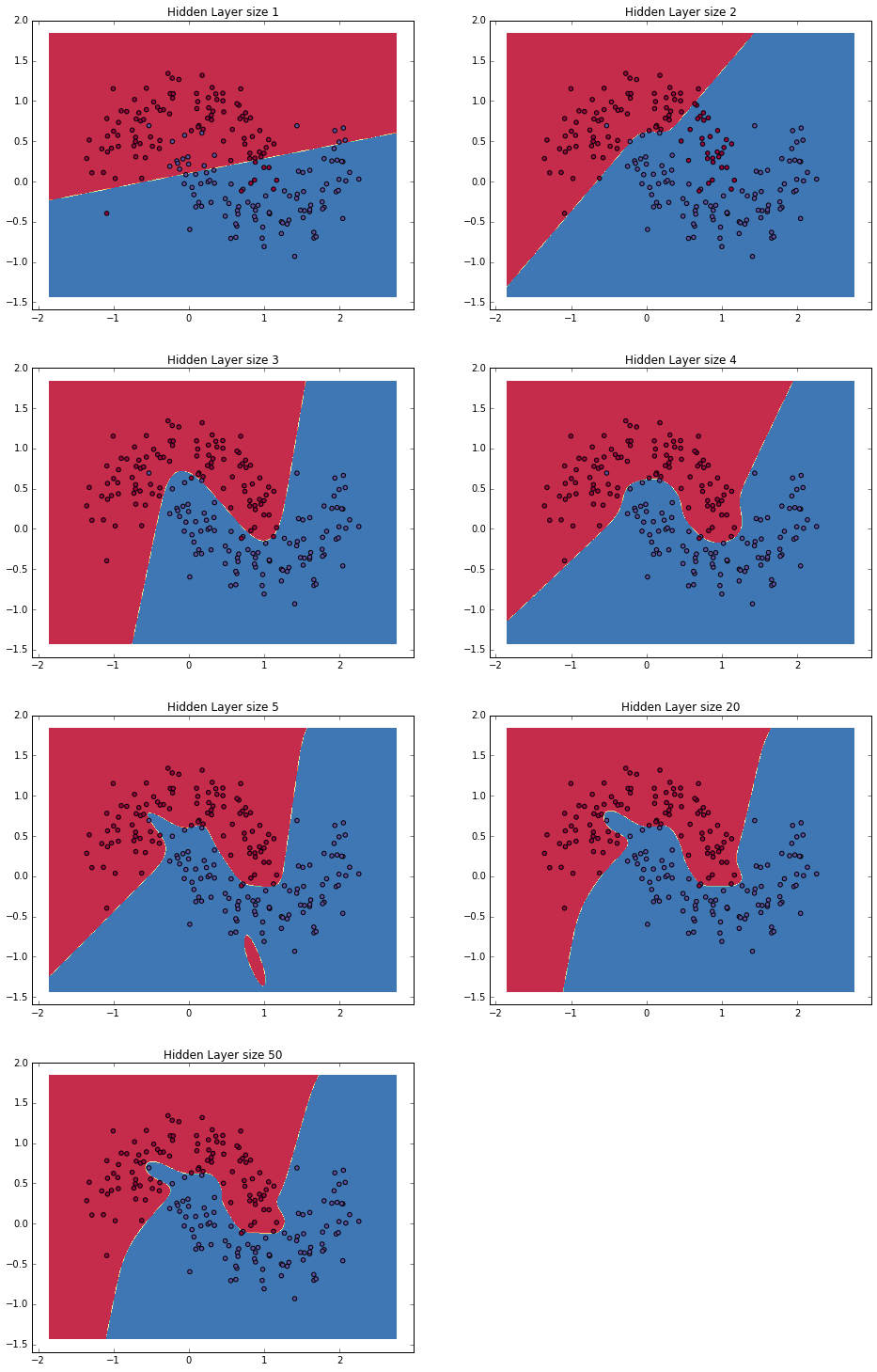
Adding more nodes doesn’t change results much—see the WildML post using the moon data for some nice visualizations of the boundaries being learned between the two classes for different hidden layer sizes.
So, a hidden layer does the trick! Let’s see what happens with the saturn data.
$ python hidden.py --train simdata/saturn_data_train.csv --test simdata/saturn_data_eval.csv --num_epochs 50 --num_hidden 2
Accuracy: 0.76
With just two hidden nodes, we already have a substantial boost from the 45% achieved by softmax regression. With 15 hidden nodes, we get 100% accuracy. There is considerable variation from run to run (due to random initialization). As with the moon data, there is less variation as nodes are added. Here’s a plot showing the increase in performance from 1 to 15 nodes, including ten accuracy measurements for each node count.
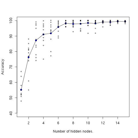
The line through the middle is the average accuracy measurement for each node count.
Initialization and activation functions are important
My first attempt at doing a network with a hidden layer was to merge what I had done in softmax.py with the network in mnist.py, provided with TensorFlow tutorials. This was a useful exercise to get a better feel for the TensorFlow Python API, and helped me understand the programming model much better. However, I found that I needed to have upwards of 25 or more hidden nodes in order to reliably get >96% accuracy on the moon data.
I then looked back at the WildML moon example and figured something was quite wrong since just three hidden nodes were sufficient there. The differences were that the MNIST example initializes its hidden layers with truncated normals instead of normals divided by the square root of the input size, initializes biases at 0.1 instead of 0 and uses ReLU activations instead of tanh. By switching to Xavier initialization (using Delip’s handy function), 0 biases, and tanh, everything worked as in the WildML example. I’m including my initial version in the repo as truncnorm_hidden.py so that others can see the difference and play around with it. (It turns out that what matters most is the initialization of the weights.)
This is a simple example of what is often discussed with deep learning methods: they can work amazingly well, but they are very sensitive to initialization and choices about the sizes of layers, activation functions, and the influence of these choices on each other. They are a very powerful set of techniques, but they (still) require finesse and understanding, compared to, say, many linear modeling toolkits that can effectively be used as black boxes these days.
Conclusion
I walked away from this exercise very encouraged! I’ve been programming in Scala mostly for the last five years, so it required dusting off my Python (which I taught in my classes at UT Austin from 2005-2011, e.g. Computational Linguistics I and Natural Language Processing), but I found it quite straightforward. Since I work primarily with language processing tasks, I’m perfectly happy with Python since it’s a great language for munging language data into the inputs needed by packages like TensorFlow. Also, Python works well as a DSL for working with deep learning (it seems like there is a new Python deep learning package announced every week these days). It took me less than four hours to go through initial examples, and then build the softmax and hidden networks and apply them to the three data sets. (And a bunch of that time was me remembering how to do things in Python.)
I’m now looking forward to trying deep learning models, especially convnets and LSTM’s, on language and image tasks. I’m also going to go back to my Scala code for trying out Deeplearning4J to see if I can get these simulation examples to run as I’ve shown here with TensorFlow. (I would welcome pull requests if someone else gets to that first!) As a person who works primarily on the JVM, it would be very handy to be able to work with DL4J as well.
After that, maybe I’ll write out the re-occurring rant going on in my head about deep learning not removing the need for feature engineering (as many backpropagandists seem to like to claim), but instead changing the nature of feature engineering, as well as providing a really cool set of new capabilities and tricks.
